Plotting

Section 2.5 Plotting

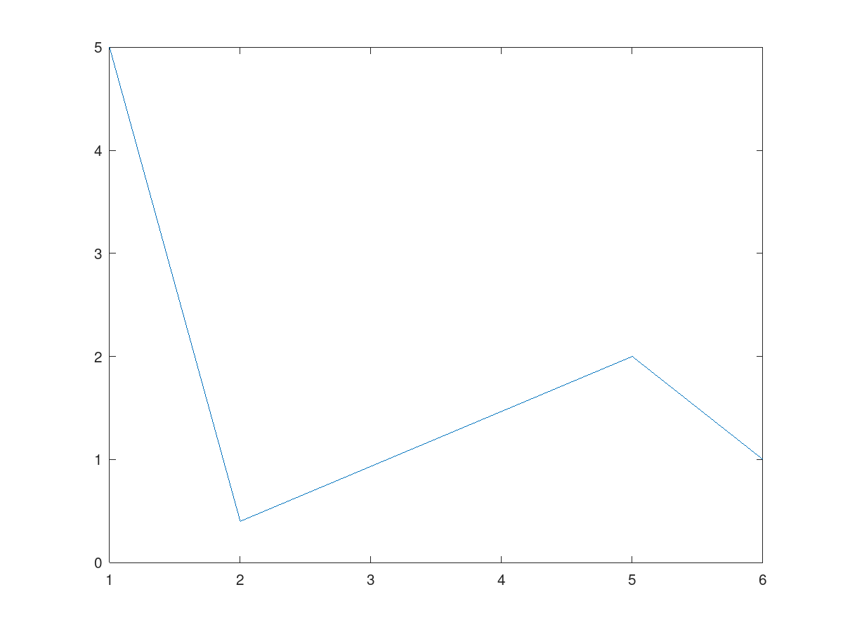
The command plot(x, y) receives two vectors: the first has x-coordinates of the points to be shown, the second has y-coordinates. It also connects these points by lines. So, for example,

plot([1 2 5 6], [5 0.4 2 1])

produces the following plot:

🔗

Figure 2.5.1. A plot based on four points
🔗

Sometimes we do not want to connect the points by a line: treating them as individual data points rather than representative of some function \(y = f(x)\text{.}\) If so,

plot([1 2 5 6], [5 0.4 2 1], '*')

simply puts an asterisk * for each point, without connecting them.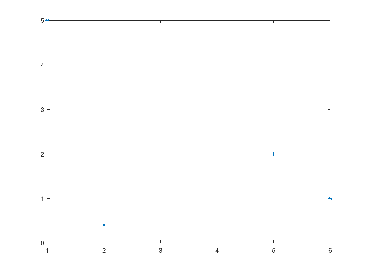

🔗

Figure 2.5.2. Four points (two are hard to see because of the axes)
🔗

Let us plot the function \(y = x^3 e^{-2x}\) on the interval \([0, 3]\text{:}\)

🔗

x = 0:0.1:3;
y = x.^3 .* exp(-2*x);
plot(x, y)

In the first line, I chose 0.1 as the step size for the x-interval. It would be a mistake to use x = 0:3 because the step size of 1 unit would make a very rough (low-resolution) plot with only four points used. The step size could be 0.01 instead: we may get smoother graph at the expense of more computations. The second line compute the y-values. Consider the following:

The period in x.^3 is required to have elementwise power operation

🔗
We do not need a period in -2*x because multiplying a vector by a scalar already works elementwise. There is no difference between -2*x and -2.*x

🔗
We need .* to multiply two vectors elementwise.

🔗
Whitespace around .* is not necessary but some people find x.^3.*exp(-2*x) harder to read because 3. looks like a decimal dot after 3.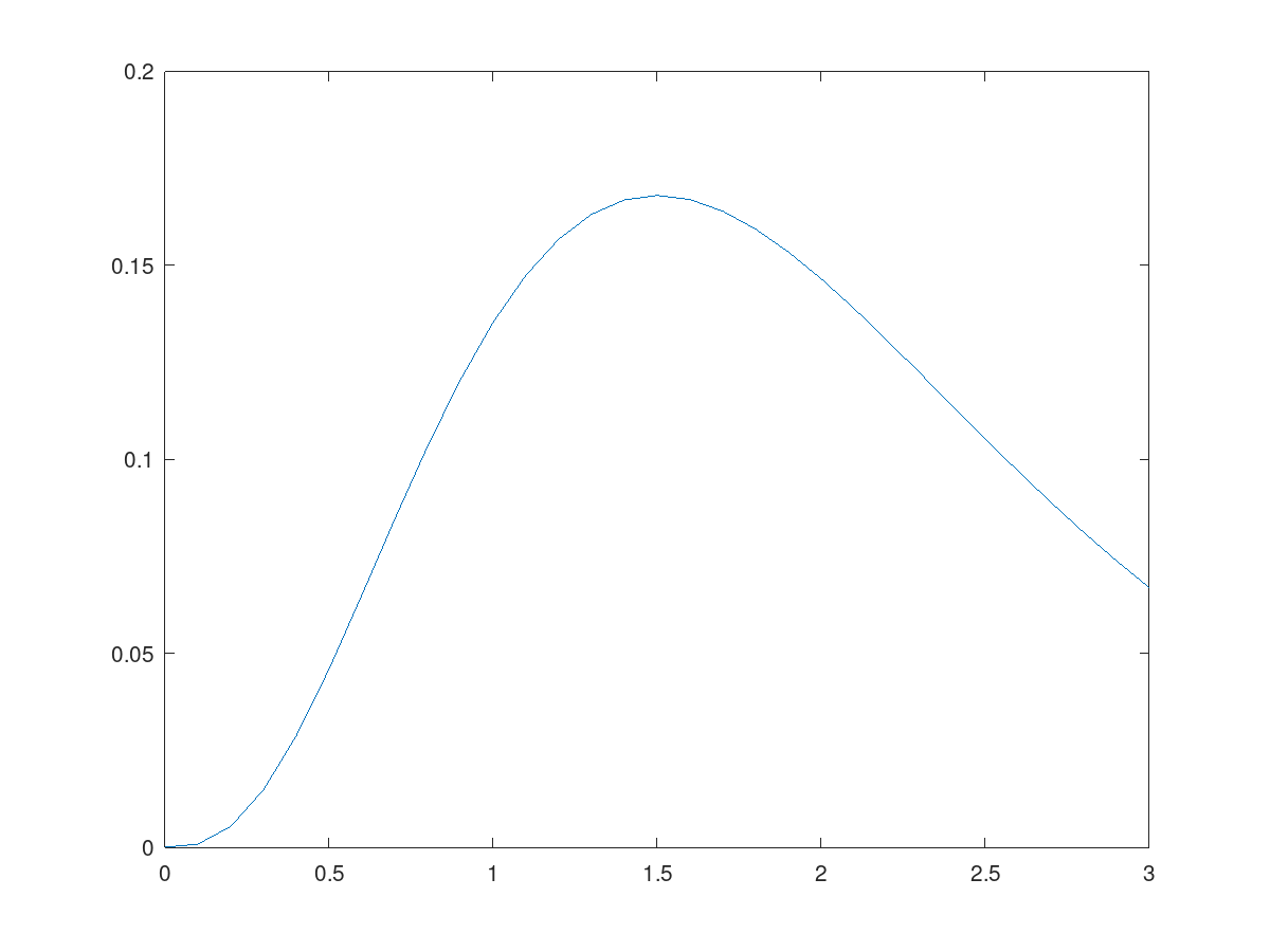

🔗

🔗

Figure 2.5.3. Plot of the function \(y = x^3 e^{-2x}\) on the interval \([0, 3]\)
🔗

Specifying the x-values by choosing step size like in x = 0:0.1:3 can be tedious, because the same step size would not work as well for the intervals \([2, 2.04]\) or for \([0, 50000]\text{.}\) The command linspace can be more convenient: linspace(a, b, n) creates a vector with n uniformly spaced numbers from a to b. Usually, 500 points are enough for a smooth plot, so one can reasonably use x = linspace(a, b, 500) for plots no matter how small or large the interval \([a, b]\) is.

🔗

Example 2.5.4. Parametric plot.

Draw the curve with parametric equations

\begin{align*} x \amp = t\cos t\\ y \amp = t\sin t \end{align*}

where \(0 \le t \le 20\text{.}\)

🔗

Answer.

t = linspace(0, 20, 500);
plot(t.*cos(t), t.*sin(t))

This curve is called the Archimedean spiral.

🔗

Prev Top Next