Section 23.1 Piecewise linear interpolation
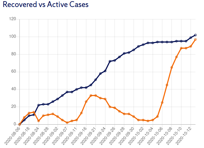
The current version of SU COVID dashboard uses piecewise linear interpolation. Geometrically this concept is clear: connect the points by straight lines, which is also what Matlab’s
plot does.
Formally, piecewise linear interpolation means that given some points \(a=x_1 \lt x_2 \lt \cdots \lt x_n = b\) on an interval \([a, b]\) and corresponding y-values \(y_1, \dots, y_n\text{,}\) we define a function \(S\colon [a, b]\to \mathbb R\) by the piecewise formula
\begin{equation}
S(x) = y_k + \frac{y_{k+1}-y_k}{x_{k+1} - x_{k}} (x - x_k),\quad x_{k}\le x\le x_{k+1}\tag{23.1.1}
\end{equation}
where the right hand side is a linear function through two points \((x_{k}, y_k)\) and \((x_{k+1}, y_{k+1})\text{.}\) So, instead of \(1\) interpolating polynomial of degree \(n-1\) we use \(n-1\) polynomials of degree \(1\text{.}\) The function \(S\) is a spline of degree 1 meaning it is a piecewise function where the pieces are polynomials of degree 1.
A more abstract approach to the construction of degree 1 spline is as follows:
-
We have \(n-1\) subintervals between \(n\) data points.
-
On each subinterval we choose a degree 1 polynomial; this means we have \(2(n-1)\) coefficients to choose.
-
But we want to spline to be continuous, so the values at each interior data point from the left and from the right must match. There are \(n-2\) interior data points, so the continuity imposes \(n-2\) equations.
-
Finally, the spline must pass through each of \(n\) data points. This adds \(n\) equations.
-
The total is \(n-2+n=2n-2\) equations with \(2(n-1) = 2n-2\) unknowns, so we expect (and get) a unique solution.
There are infinitely many ways to connect given data points. The function (23.1.1) does so by a curve of minimal length, meaning that the graph of \(S\) is the shortest curve passing through the given data points. This is a reasonable way of connecting the points, but not necessarily the best or most natural way. The corners at the data points do not look natural. The piecewise linear graph does not give much insight into the rate of change of the function because it treats the rate as constant on each interval. For example, given the function values
x = 1:5;
y = [8 5.5 5.3333 5.75 6.4];
what is the derivative of the function at \(x = 2\text{?}\) Differentiating the piecewise linear interpolant gives some information but not much. Another question one might ask is: where is the minimum of this function? The minimum of piecewise linear interpolant is exactly at \(x=3\) but we understand the actual function probably has its minimum between \(2\) and \(3\text{.}\)
