Newton's method

Section 9.1 Newton's method

The idea of Newton's method is geometrically natural. We want to solve

$f(x) = 0$ but since

$f$ may be complicated, we replace it by its linear approximation (tangent line at a certain point). The resulting linear equation is easy to solve. Of course, its solution is probably not a solution of the original equation, but perhaps it is close to it. The process repeats, using the previously found solution as a new point at which to draw a tangent line. A static image of this process is below. Interactive visualization is also available.

🔗
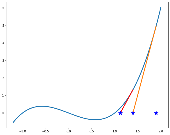
Figure 9.1.1. Two steps of Newton's method

🔗

Formally, the linear approximation to

$f$ at a point

$x$ is

$f(x+h) \approx f(x) + f'(x)h\text{.}$ Equating the right hand side to 0 we find

$h = -f(x)/f'(x)$ which means that the point where the tangent line at

$x$ meets the line

$y=0$ is

$x + h = x - f(x)/f'(x)\text{.}$ Therefore, we can express Newton's method as iteration of the function

$\begin{equation*} g(x) = x - \frac{f(x)}{f'(x)} = \frac{xf'(x) -f(x)}{f'(x)} \end{equation*}$

🔗

Note that any point where

$f(x) = 0$ and

$f'(x)\ne 0$ is a fixed point of

$g\text{.}$ In fact, it is a super-attracting point of

$g$ because

$\begin{equation*} g'(x) = 1 - \frac{f'(x)f'(x) - f(x)f''(x)}{(f'(x))^2} = \frac{f(x)f''(x)}{(f'(x))^2} \end{equation*}$

🔗

which is zero when

$f(x) = 0\text{.}$

🔗

Example 9.1.2. Find and simplify the function $g$ of Newton's method.

Given $f(x) = x^3 - x\text{,}$ find and simplify the function $g(x) = x - f(x)/f'(x)\text{.}$

Solution

Bringing $g$ to common denominator often helps:

\begin{equation*} g(x) = \frac{xf'(x) -f(x)}{f'(x)} = \frac{x(3x^2-1) - (x^3-x)}{3x^2-1} = \frac{2x^3}{3x^2-1} \end{equation*}

🔗

Once we have the function

$g\text{,}$ the rest of the process is the same as in Chapter 8, in particular in Example 8.2.1. Changing the first two lines of that program to

g = @(x) 2*x^3/(3*x^2-1); 
x0 = 0.6;

🔗

we get “Found x = 1 after 11 steps”. If the starting point is different, the process may converge to a different root of the equation

$x^3-x = 0\text{.}$ For example with x0 = 0.57 we get “Found x = -1 after 14 steps”. A small change of initial condition produced a rather different solution; we went from finding x = 1 to finding x = -1. The pattern of what starting points produce which solution can be very complicated: see the illustrations on Wikipedia page Newton fractal.

Section 9.1 Newton's method

Example 9.1.2. Find and simplify the function gg of Newton's method.

Example 9.1.2. Find and simplify the function $g$ of Newton's method.