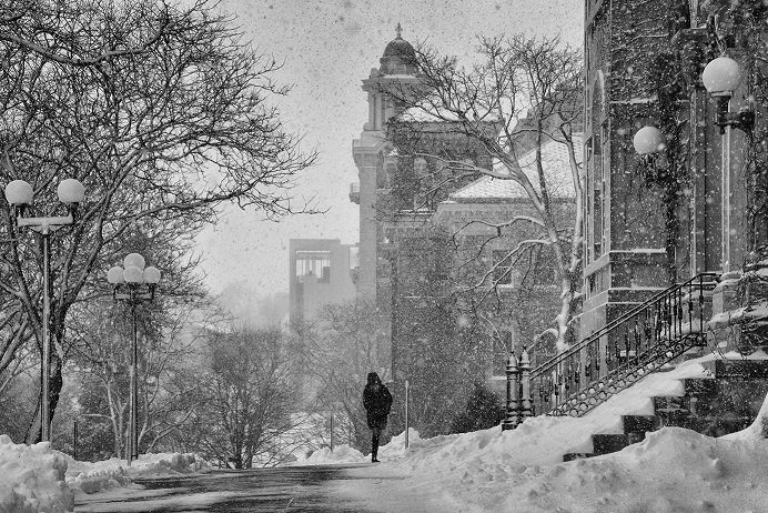
Section 26.2 Two-dimensional DFT

Since images are two-dimensional (considering either grayscale images, or working with each color channel separately), they can be processed using the two-dimensional version of Discrete Fourier Transform, implemented in Matlab as fft2 and (inverse) ifft2. The formulas for 2D transform follow the same logic as one-dimensional formulas (25.3.2) and (25.3.3). Namely, the 2D Fourier coefficients of a given matrix \((z_{k\ell})\) with indices \(k=0, \dots, m-1\text{,}\) \(\ell=0, \dots, n-1\) are computed as:

\begin{equation} c_{pq} = \sum_{k=0}^{m-1} \sum_{\ell=0}^{n-1} z_{k \ell} \exp(-2\pi i k p/m) \exp(-2\pi i \ell q/n) \label{eq-fourier-coefficients-discrete-2d}\tag{26.2.1} \end{equation}

The matrix is reconstructed from its coefficients by inverse transform

\begin{equation} z_{k\ell} = \frac{1}{mn} \sum_{p=0}^{m-1}\sum_{q=0}^{n-1} c_{pq} \exp(2\pi i kp/m) \exp(2\pi i \ell q/n) \label{eq-fourier-sum-discrete-2d}\tag{26.2.2} \end{equation}

The fact that Matlab indices begin with 1 means they have to be shifted by 1 in the above formulas, but since we will just use fft2 and (inverse) ifft2, we will not worry about this.

Let us try this with the grayscale version of the winter image, saved here as a PNG file for lossless compression.

Figure 26.2.1. Grayscale PNG image

After loading the image with im = imread('winter.png'), check this is a matrix (no separate channels for colors). Try fc = fft2(im); which produces a matrix of the same size but with complex entries. It is not easy to understand all of it. Small pieces can be inspected with fc(1:5, 1:5) for example: when doing this, notice the special role of fc(1, 1), the upper left number. A histogram can help visualize the distribution of the magnitudes of Fourier coefficients: histogram(abs(fc(:)), 50). (Recall that fc(:) means flattening a matrix to a vector.) Looks like nearly all coefficients are much smaller than the largest ones.

We can set all small Fourier coefficients (less than some threshold thr) to zero using fc(abs(fc) < thr) = 0;. One way to determine the threshold reasonably is to use percentiles: for example,

thr = prctile(abs(fc(:)), 75);

returns the number thr such that 75 percent of Fourier coefficients are less than it, and the other are greater (in absolute value).

Given a percentage p, such as 75, compress the “winter” image by setting p percent of its Fourier coefficients to zero.

Solution
p = 75;
im = imread('winter.png');
fc = fft2(im);
thr = prctile(abs(fc(:)), p);
fc(abs(fc) < thr) = 0;
im2 = uint8(real(ifft2(fc)));
imshow(im2)

The inverse Fourier transform may have imaginary part due to the truncation of Fourier coefficients and rounding errors in computations. This imaginary part is removed with real. The result is converted to unsigned 8-bit integers with uint8.

The JPEG compression algorithm is based on the Fourier Transform but differs from the above example in several ways:

  • It divides the image into 8×8 pixel blocks and operates on each block separately.
  • It uses Discrete Cosine Transform in which the role of complex exponentials \(\exp(2\pi i k/m)\) is played by cosine functions \(\cos(2\pi k/m)\text{.}\) This improves the efficiency and eliminates the appearance of complex numbers.
  • In addition to setting small Fourier coefficients to 0, it quantizes the other ones: rounds to the nearest integer, or nearest multiple of 5, etc.
  • Since setting many elements to 0 does not by itself make a matrix smaller, the final step of the process is running a lossless compression algorithm which exploits the existence of many equal entries in the matrix.