Numerical Methods with Programming

Section 23.2 Cubic splines

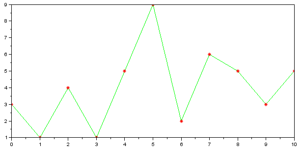
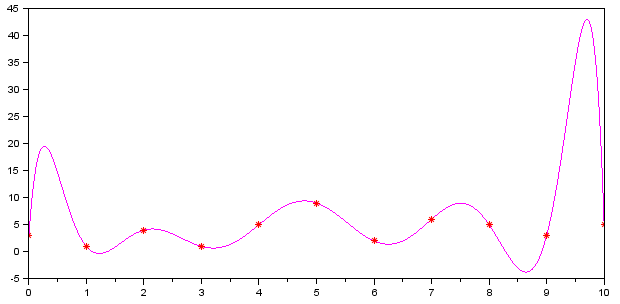
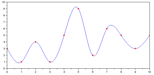
A cubic spline is a function \(S\) that is piecewise a degree 3 polynomial, and such that \(S, S', S''\) are continuous (have the same value from both sides at the points where pieces meet). In our context of fitting to data points \((x_k, y_k)\text{,}\) \(k=1, \dots, n\text{,}\) it is natural to have each cubic polynomial defined on \([x_{k}, x_{k+1}]\text{.}\) The continuity of first and second derivatives means that the graph of a cubic spline has no corners of sudden changes of curvature, it flows quite naturally. Compare the plots below, for the same data set.

Cubic splines were also used by the first version of SU COVID dashboard:

Let us count unknowns and equations involved in the construction of a cubic spline.

• We have \(n-1\) subintervals between \(n\) data points.
• On each subinterval we choose a degree 3 polynomial; this means we have \(4(n-1)\) coefficients to choose.
• In order for \(S, S', S''\) to be continuous at each of \(n-2\) interior data points, there are \(3(n-2)\) equations to satisfy.
• The spline must pass through each of \(n\) data points. This adds \(n\) equations.
• The total is \(3(n-2)+n=4n-6\) equations with \(4(n-1)=4n-4\) unknowns, so need two more equations to make the solution unique.

When discussing spline coefficients, it should be noted they are not necessarily the coefficients of powers of \(x\text{.}\) It is more natural and numerically safer to represent the spline on each subinterval \([x_k, x_{k+1}]\) in terms of the powers of \((x-x_k)\text{.}\) That is,

where the coefficients \(a_k, b_k, c_k, d_k\) are to be determined. Of course, \(D_k=y_k\) but to find the rest one needs to solve a linear system.

Here are three different ways to add two more equations to the linear system for coefficients; they result in three different kinds of cubic splines:

• Require \(S''(a) = 0 = S''(b)\text{.}\) This is a “natural spline”.
• Require \(S'(a) = p\) and \(S'(b)=q\) for some values \(p, q\text{.}\) This is a “clamped spline”.
• Require \(S'''\) to be continuous at \(x_2\) and at \(x_{n-1}\text{.}\) This is a “not-a-knot spline”.

This terminology needs some explanation. The word spline used to refer to a long thin strip of flexible material (e.g., metal) which, if constrained at several points, assumes the shape of a smooth curve passing through these points. Unlike an elastic band which minimizes its length (creating a piecewise linear shape), the spline minimizes its bending energy. A mathematical idealization of the bending energy of a curve \(y=f(x)\) is the integral \(\int_a^b f''(x)^2\,dx\text{.}\) It can be shown that among all functions (of whatever form) that satisfy the constraints \(f(x_k)=y_k\text{,}\) the “natural spline” has the smallest value of \(\int_a^b f''(x)^2\,dx\text{.}\) This attractive mathematical property earned it the “natural” name… but upon further reflection, the boundary conditions \(S''(a) = 0 = S''(b)\) are actually not that natural. If we are interpolating some smooth function \(y=f(x)\text{,}\) there is no reason to assume that \(f''\) happens to be \(0\) at the endpoints.

Clamped splines refer to holding the ends of the metal strip with a clamp, which restricts not only its position but also the angle. This spline is useful for for modeling a problem with boundary conditions on the derivative.

The knots of a spline are the transition points where it turns from one polynomial to another. These are often, but not always, the points \(x_k\) from the given data. Requiring \(S'''\) to be continuous at \(x_2\) implies we have the same polynomial on both intervals \([x_1, x_2]\) and \([x_2, x_3]\) (why?), and therefore \(x_2\) is not a knot for this spline. Same for \(x_{n-1}\text{.}\) The not-a-knot condition is the standard choice when we do not have any reason to impose other conditions.