Section 22.2 Chebyshev polynomials and interpolation
In Chapter 15 we studied Legendre polynomials \(P_n\) which are orthogonal on the interval \([-1, 1]\) in the sense that \(\int_{-1}^1 P_n(x)P_k(x)\,dx = 0\) when \(n\ne k\text{.}\) We also use Laguerre polynomials \(L_n\) which are orthogonal on \([0, \infty)\) with the weight function \(e^{-x}\text{,}\) meaning that \(\int_{-1}^1 L_n(x)L_k(x)\,e^{-x}\,dx = 0\) when \(n\ne k\text{.}\) The Chebyshev polynomials \(T_n\) are orthogonal on the interval \([-1, 1]\) with the weight function \(1/\sqrt{1-x^2}\text{,}\) meaning that
As for other families of orthogonal polynomials, we have a recursive formula for Chebyshev polynomials: starting with \(T_0(x)=1\) and \(T_1(x) =x\) we can compute the rest as
The recursion is simpler than for \(P_n\) or \(L_n\text{:}\) there is no division, so all polynomials \(T_n\) have integer coefficients.
Example 22.2.1. Plot Chebyshev polynomials \(T_n\).
Recursively find the coefficients of Chebyshev polynomials \(T_n\) for \(n\le 6\text{.}\) Plot all of them on the interval \([-1, 1]\text{.}\)
This is a straightforward modification of Example 15.4.1.
p = [1]; q = [1 0]; x = linspace(-1, 1, 1000); hold on plot(x, polyval(p, x), x, polyval(q, x)); for n = 1:5 r = 2*[q 0] - [0 0 p]; p = q; q = r; plot(x, polyval(r, x)) end hold off
Example 22.2.1 indicates that Chebyshev polynomials oscillate between \(-1\) and \(1\) on the interval \([-1, 1]\text{.}\) The following remarkable identity confirms this observation:
for all \(\theta\in\mathbb R\text{.}\) The proof is by induction. Base of induction is \(n=0, 1\text{:}\) for \(T_0(x)=1\) and \(T_1(x)=x\) the validity of (22.2.2) is obvious. For the inductive step, assume (22.2.2) holds for \(T_0, \dots, T_n\) and use (22.2.1):
where the second step involves the identity
The right hand side of (22.2.2) is zero when \(n\theta\) is an odd multiple of \(\pi/2\text{,}\) hence \(\theta = (2k-1)\frac{\pi}{2n}\text{.}\) Plugging \(k=1, \dots, n\) we find that
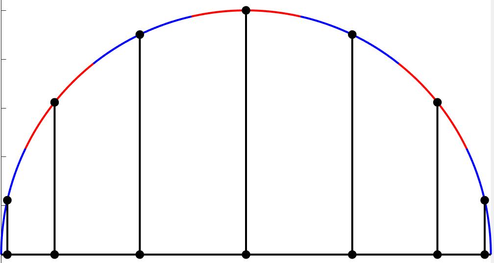
and since the polynomial \(T_n\) can have at most \(n\) real roots, these are all of its roots. They are easy to visualize: draw a semi-circle with interval \([a, b]\) as diameter, divide it into \(n\) equal arcs, and project the midpoint of each arc back to the interval.
The recursive formula shows that the leading coefficient of \(T_n\) is \(2^{n-1}\text{.}\) Therefore,
where \(x_1, \dots, x_n\) are the roots (22.2.3). It follows that the absolute value of the product \(\prod_{k=1}^n (x-x_k)\) is bounded by \(2^{1-n}\text{.}\) It can be proved that \(2^{1-n}\) is as small as one can get for any choice of \(n\) points on the interval \([-1, 1]\text{.}\) This suggests that Chebyshev points should work well for polynomial interpolation, and they do. Let us re-do Example 21.2.2 with random data to illustrate this.
Example 22.2.3. An interpolating polynomial using Chebyshev points.
Let \(x_1, \dots, x_{10}\) be the roots of \(T_{10}\text{.}\) Choose \(y_k\) randomly from the standard normal distribution, and draw the interpolating polynomial through the points \((x_k, y_k)\text{.}\)
The only change to Example 21.2.2 is replacing the x-coordinates.
n = 10; x = cos((2*(1:n)-1)*pi/(2*n)); y = randn(1, n); w = ones(1, n); for k = 1:n for j = 1:n if j ~= k w(k) = w(k)/(x(k)-x(j)); end end end p = @(t) (y.*w*(t - x').^(-1)) ./ (w*(t - x').^(-1)); t = linspace(min(x)-0.01, max(x)+0.01, 1000); plot(t, p(t), x, y, 'r*')
Running the code Example 22.2.3 several times, we see that the interpolating polynomial behaves reasonably, without unnatural oscillations that come from interpolating at equally spaced points.