Section 35.4 Duality in optimal transportation
This is an optional section, feel free to skip it.
The book Topics in Optimal Transportation by Cédric Villani presents the following illustration of duality, credited by the author to Luis Caffarelli. In this book the duality theorem is named after Leonid Kantorovich.
Suppose for instance that you are both a mathematician and an industrialist, and want to transfer a huge amount of coal from your mines to your factories. You can hire trucks to do this transportation problem, but you have to pay them \(c(X, Y)\) for each ton of coal which is transported from place \(X\) to place \(Y\text{.}\) Both the amount of coal which you can extract from each mine, and the amount which each factory should receive, are fixed. As you are trying to […] minimize the price you have to pay, another mathematician comes to you and tells you:“My friend, let me handle this for you: I will ship all your coal with my own trucks and you won’t have to worry about what goes where. I will just set a price \(\varphi(X)\) for loading one ton of coal at place \(X\text{,}\) and a price \(\psi(Y)\) for unloading it at destination \(Y\text{.}\) I will set the prices in such a way that your financial interest will be to let me handle all your transportation! Indeed, you can check very easily that for any \(X\) and \(Y\text{,}\) the sum \(\varphi(X)+\psi(Y)\) will always be \(\le c(X, Y)\) (in order to achieve this goal, I am even ready to give financial compensations for some places, in the form of negative prices!)”.Of course you accept the deal. Now, what Kantorovich’s duality tells you is that if this shipper is clever enough, then he can arrange the prices in such a way that you will pay […] as much as you would have been ready to spend by the other method.
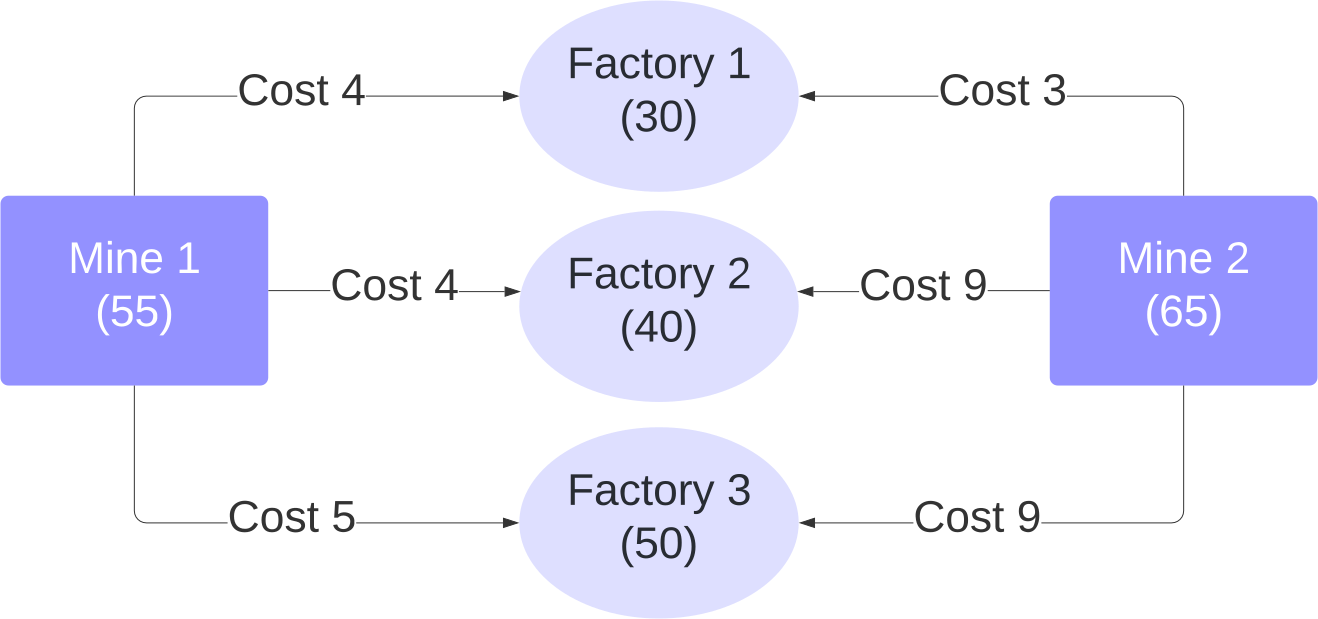
What form of duality is this, and where do negative prices come from? This is an example of asymmetric duality, where the primal problem is of type EN (moving nonnegative amounts of coal, which must add up exactly to what is available or required), and the dual problem is of type IR (setting possibly negative prices, allowing for inequalities \(\varphi(X)+\psi(Y) \le c(X, Y)\)). Here is a concrete example with two coal mines and three factories: the amounts of production, consumption, and transportation costs per unit are stated on the diagram.

Let \(x_1, x_2, x_3\) be the amounts sent from Mine 1 to Factories 1, 2, 3. Also let \(x_4, x_5, x_6\) be the amounts sent from Mine 2 to Factories 1, 2, 3. The constraints can be expressed in matrix form as \(A\mathbf x = \mathbf b\) where
\begin{equation*}
A = \begin{pmatrix}
1 & 1 & 1 & 0 & 0 & 0 \\
0 & 0 & 0 & 1 & 1 & 1 \\
1 & 0 & 0 & 1 & 0 & 0 \\
0 & 1 & 0 & 0 & 1 & 0 \\
0 & 0 & 1 & 0 & 0 & 1 \\
\end{pmatrix} \qquad
\mathbf b = \begin{pmatrix} 55 \\ 65 \\ 30 \\ 40 \\ 50 \end{pmatrix}
\end{equation*}
The coefficients of objective functions are the unit cost, \(\mathbf c^T = (4, 4, 5, 3, 9, 9)\text{.}\) And of course, \(\mathbf x\ge 0\text{:}\) even if we wanted to allow factories to send excess coal back to a mine, this would not fit the LP model since the cost of such transportation would not be negative.
To solve the linear program in Matlab, we use expanded syntax of
linprog:x = linprog(c, A, b, Aeq, beq, lb, ub);
where the additional parameters
Aeq, beq express a linear system of equality constraints, and the vectors lb, ub provide lower and upper bounds on the variables. In our case, we do not have any inequality constraints so the second and third arguments are empty. The last one is omitted since we do not have upper bounds.A = [1 1 1 0 0 0; 0 0 0 1 1 1; 1 0 0 1 0 0; 0 1 0 0 1 0; 0 0 1 0 0 1];
b = [55; 65; 30; 40; 50];
c = [4; 4; 5; 3; 9; 9];
x = linprog(c, [], [], A, b, zeros(6, 1));
fprintf('Found x = (%g, %g, %g, %g, %g, %g) with total cost %g \n', x, c'*x);
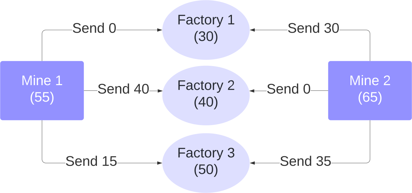
The solution is pictured below.

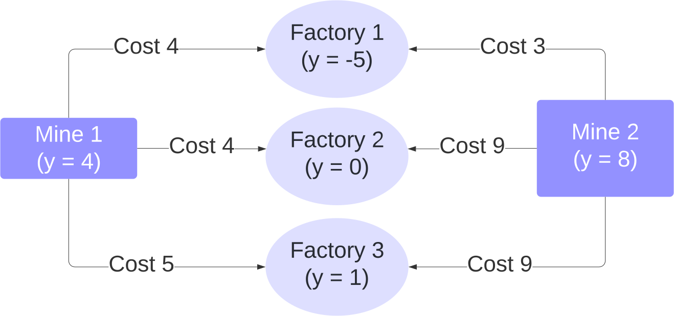
According to Section 35.2, the dual problem is to maximize \(\mathbf b^T \mathbf y\) subject to the constraint \(A^T \mathbf y\le \mathbf c\text{.}\) The vector \(\mathbf y\) expresses the pricing policy of the second mathematician (or a shipping company): they charge \(y_1, y_2\) to load a unit of coal at Mines 1, 2, and also charge \(y_3, y_4, y_5\) to unload it at Factories 1, 2, 3. The constraint \(A^T \mathbf y\le \mathbf c\) is what the company needs to win your business, and the amount maximized, \(\mathbf b^T \mathbf y\text{,}\) is their total revenue.
y = linprog(-b, A', c);
fprintf('Found y = (%g, %g, %g, %g, %g) with total revenue %g \n', y, b'*y);
The solution is pictured below. The costs \(\mathbf c\) are included to demonstrate that the constraints are satisfied. The message “Found y = (4, 8, -5, 0, 1) with total revenue 640” shows that the company will subsidize unloading at Factory 1 in order to maximize its revenue while undercutting any competition.

If we required the loading/unloading prices to be nonnegative, the transportation company would not be able to realize the same revenue.
y = linprog(-b, A', c, [], [], zeros(5, 1));
fprintf('Found y = (%g, %g, %g, %g, %g) with total revenue %g \n', y, b'*y);
“Found y = (0, 3, 0, 4, 5) with total revenue 605”
