1.
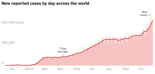
The graph shows three stages of accelerated growth: March-April, June-July, and from October onward. Since the total reflects the spread of disease in different regions, it is natural that it looks like the sum of different logistic curves.
Accordingly, we try modeling this by the sum of three logistic curves. To reduce the amount of data, we use the 7-day averages reported on the 1st, 11th, and 21th of every month, from March 1 to November 21. These 27 data values (measured in thousands) are below.
y = [1 4 21 67 80 79 77 85 94 110 126 148 180 205 230 257 259 254 265 267 292 295 337 389 503 573 588];
The corresponding x-values are simply
x = 1:numel(y). Run plot(x, y, '*') to visualize the data: this will help with choosing initial parameters, as described below.
High-dimensional optimization is difficult, and
fminsearch will need your help in the form of a good initial point (ones(9, 1) is not good enough). The logistic equation (29.2.1) leads to the 9-parameter model
\begin{equation}
y = \frac{M_1}{1 + e^{-(x-a_1)/s_1}} + \frac{M_2}{1 + e^{-(x-a_2)/s_2}} + \frac{M_3}{1 + e^{-(x-a_3)/s_3}}\tag{29.4.1}
\end{equation}
Reasonable initial guesses would be:
-
\(a_1, a_2, a_3\) are the x-values of places where the three “waves” are the steepest
-
\(M_1, M_2, M_3\) are the sizes of the three waves (how much each of them adds to the total)
-
\(s_1, s_2, s_3\) are about a tenth of the non-flat span of the wave.
Follow the examples such as Example 29.2.1 in plotting the best-fitting curve together with the data. Since the main interest in building a model like this is to predict future development, extend the curve by a month into the future (this means 3 units on x-axis). What does it predict for December 21?
