Despite the presence of absolute value and \(\max\text{,}\) both potential sources of non-smoothness, the function (24.2.2) is differentiable and even twice differentiable, with continuous \(B''\text{.}\) (This qualifies it as a cubic spline.) Why is this so?
Section 24.2 Hat functions and B-splines
We look for a way to smoothly model the data while avoiding the issues in Section 24.1. To simplify the computations, assume the x-values are equally spaced, which means that after shifting and scaling we can assume \(x_k=k\) for \(k=1, \dots, n\text{.}\) Then the linear interpolation can be expressed as the sum
\begin{equation}
L(x) = \sum_{k=1}^n y_k H(x-k)\tag{24.2.1}
\end{equation}
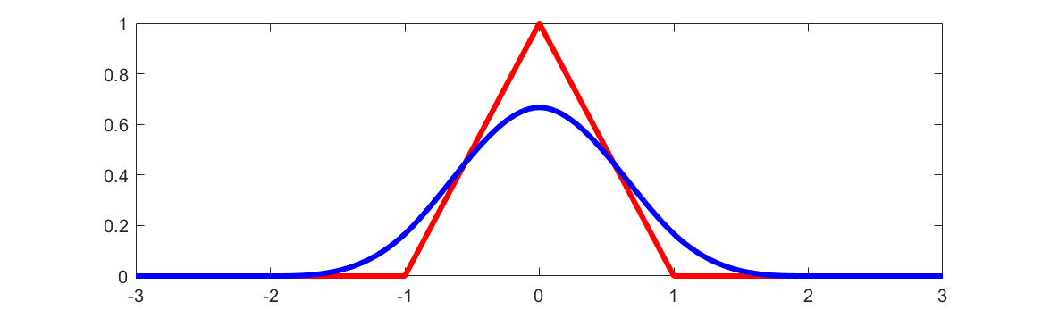
where \(H(x) = \max(0, 1-|x|)\) is a function whose graph is a triangle with base \([-1,1]\text{.}\) Functions like \(H\) are sometimes called the “hat functions” based on the appearance of the graph. An important feature of the functions \(H(x-k)\) is that they add up to \(1\) everywhere on the interval \([1, n]\) (why?). This ensures that interpolation of constant values \(y_1=\cdots =y_n\) produces a constant function, which is a necessary condition for the algorithm to preserve monotonicity of data.
As we know, piecewise linear interpolation lacks smoothness, and this is seen in the angular shape of the hat function (24.2.1). We would like to replace it with something of similar shape but smooth. Here is a piecewise cubic function which does the job.
\begin{equation}
B(t) = \frac16 \max(0,2-|t|)^3 - \frac23 \max(0,1-|t|)^3\tag{24.2.2}
\end{equation}
Its graph on \([-3, 3]\) is shown below, with the hat function \(H\) for comparison. In technical terms, both \(H\) and \(B\) are “cardinal B-splines” of degrees 1 and 3, respectively.
Question 24.2.2. Smoothness of cardinal B-spline.
Before considering how the smooth bump function (24.2.2) was constructed, let us try using it. One is the straightforward approach: replace \(H\) with \(B\) in the formula (24.2.1), obtaining a cubic spline
\begin{equation}
S(x) = \sum_{k=1}^n y_k B(x-k)\tag{24.2.3}
\end{equation}
The first thing to notice is that the spline \(S\) does not interpolate the data. Indeed, from (24.2.2) we have \(B(0)=2/3\) and \(B(\pm 1)=1/6\text{,}\) which implies that
\begin{equation}
S(x_k) = \frac{y_{k-1} + 4y_k + y_{k+1}}{6}\tag{24.2.4}
\end{equation}
which is a Simpson-style averaging of neighboring \(y\)-values. It may be disappointing not to have \(S(x_k)=y_k\) but on the other hand, averaging raw data values within some moving window is a standard approach to eliminating noise and short-term fluctuations.
It is also possible to derive an interpolating spline as a linear combination of bumps \(B(x-k)\text{,}\) by solving a simple linear system. Indeed, we can find the coefficients \(c_1, \dots, c_n\) such that
\begin{equation*}
\sum_{k=1}^n c_k B(x-k) = y_k,\quad k=1,\dots, n
\end{equation*}
by solving the system \(Ac=y\) where \(A\) is the tridiagonal matrix
\begin{equation*}
A = \frac{1}{6} \begin{pmatrix}
4 & 1 & 0 & \cdots & 0 \\
1 & 4 & 1 & \cdots & 0 \\
0 & 1 & 4 & \cdots & 0 \\
\vdots & \vdots & \vdots & \vdots & \vdots
\end{pmatrix}
\end{equation*}
But this brings back the kind of splines in Chapter 23 with the deficiencies noted earlier, so we do not pursue this approach further.
As written, the formula (24.2.3) has an issue at the boundary, where instead of averages (24.2.4) we get
\begin{equation}
S(x_1)= \frac{4y_1 + y_{2}}{6},\quad S(x_n) = \frac{y_{n-1} + 4y_n }{6}\tag{24.2.5}
\end{equation}
because there is no \(y_0\) or \(y_{n+1}\text{.}\) This is an issue because, for example, with constant values \(y_k=1\) we get \(S(x_1)=5/6=S(x_n)\text{,}\) failing monotonicity. To fix the boundary behavior, we should extend the sum (24.2.3) with two more terms:
\begin{equation}
S(x) = \sum_{k=0}^{n+1} y_k B(x-k),\quad y_0=y_1, \ y_{n+1} = y_n\tag{24.2.6}
\end{equation}
This is typical when computing with values on a grid: sometimes our formulas refer to out-of-grid points, and instead of just ignoring such terms we should somehow extrapolate the known values outside of the grid.
Example 24.2.3. Implement cubic spline approximation.
Use the examples from Section 24.1 to demonstrate that the spline formula (24.2.6) preserves monotonicity and positivity.
Answer.
B = @(t) (1/6)*max(0, 2-abs(t)).^3 - (2/3)*max(0, 1-abs(t)).^3;
x = 1:6;
y = [0 0 1 1 2 2];
xe = [x(1)-1, x, x(end)+1];
ye = [y(1), y, y(end)];

t = linspace(min(x), max(x), 1000);
S = ye*B(t - xe');
plot(t, S, x, y, 'r*')
As discussed above, the x-y values are extended by two points to the left and right; this is what the vectors
xe and ye represent. After that, the spline is evaluating in a single vectorized computation. The plot shows a smoothly increasing function. Trying this again with y = [9 9 1 1 9 9] we get a smooth positive function.
